
Installation instructions:
1. Download PMdisp.zip by clicking here.
2. Unzip the PMdisp.zip file.
(Go to www.WinZip.com if you do not have an unzipping program installed.)
3. Run Setup.exe and follow the on-screen instructions.
4. Run PMfiber from the CIRL software program group of the Start menu.
Model Description:
This model uses the same mode coupling calculations as PMfiber and Cascade. PMFiber is a model for illustrating the state of polarization along a PM fiber, based on the division of the propagating path into small slices which are rotated in small increments. The new state of polarization is calculated after each discontinuity. The light is assumed coherent and CW resulting in a unique output state of polarization. A similar program (Cascade) is used for a string of PM components along a PM fiber where the new state of polarization is calculated after a cross coupled component.
In the case of polarization mode dispersion where the light is a pulse propagating along a fiber we consider the phase difference introduced by the small difference in the propagation constants of the birefringent axes of the fiber created by manufacturing methods, bends and stress effects. It is convenient to treat the fiber as successive lengths of weakly birefringent fiber with a specified rotation between each length. The rotation can be selected to be random, or a small incremental change to illustrate a slowly rotating fiber. The pulse travels along the birefringent axes and after each rotation of the next fiber length results in a new state of polarization and a distribution of different states along the pulse due to displacement. Depending on the model input parameters, it can be shown that the pulse simply broadens in both principal axes or there is significant displacement between axes with little broadening.
The PMD model
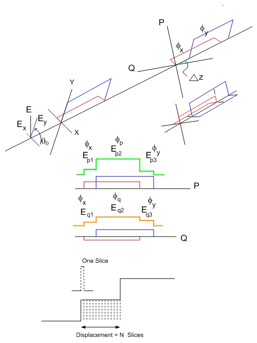
The figure shows a pulse *E* resolved into components *E_x * and *E_y * on the axes of a PM fiber. The pulse propagates a distance along the fast and slow z axes such that a displacement Dz occurs and the components have a new phase f_x and f_y (strictly at the leading edge). At this distance there is a rotation of the axes from X-Y to P-Q, and a new refractive index set N_x and N_y . The modified pulse in the P and Q axes has three distinct parts in each of the P and Q axes. It can be seen that the first part has phase f_x with amplitudes E_p1 and E_q1 , there being no overlap with the f_y component. Similarly the last part has phase f_y with amplitude E_p3 and E_q3 . The mid part has a combination of f_x and f_y resulting in f_p and f_q with amplitudes E_p2 and E_q2.
The new pulse is propagated a second distance to the next set of rotated axes with similar changes in N_x and N_y and this results in a pulse with up to five different phase and amplitude parts. Propagation for further distances (the number of iterations) gives the final graphical outputs as shown in the display. In this model the pulse is divided into a number of segments. The pulse is propagated a relatively large distance along a weakly birefringent fiber such that the displacement of the components is an integral number of the segments. The segments are made small enough to allow a large range of phase differences for each displacement. The parts of the pulse that result from several iterations can be numerous due to random displacements giving rise to many edges, or can be relatively small if the displacements are constant.
Interface:
Click here to see a screen-shot of the PM Dispersion Program.
Output:
The plot window displays three separate graphs. The first plot, Rotation and Displacement, is a representation of the displacements (shown in green) and rotations (shown in red) used in the successive PMD iterations. A flat line indicates a constant value throughout all iterations. The second plot, Power and Normalized Phase along Pulse, plots the power (in green) and the normalized phase (in red) over each segment of the pulse. The third plot, Pulse Intensity Ep Es, plots the intensity of both output components over each segment of the pulse.
Parameters:
|
|
|||